

Gradient descent sits at the heart of modern machine learning and artificial intelligence. From training deep neural networks to optimising linear regression models, it provides a systematic way to minimise an objective function through repeated, incremental updates. While the algorithm itself is conceptually simple, the theory behind its convergence is far richer. Questions about how fast gradient descent converges, under what conditions it remains stable, and why it sometimes fails are central to both academic research and practical implementation. A clear understanding of convergence theory helps practitioners design models that train reliably rather than unpredictably.
The Role of the Objective Function in Convergence
The behaviour of gradient descent is tightly coupled to the properties of the objective function being optimised. Smoothness, convexity, and curvature all influence how the algorithm progresses. When an objective function is convex and differentiable, gradient descent enjoys strong theoretical guarantees. Each iteration moves the parameters closer to the global minimum, provided the step size is chosen appropriately.
In contrast, non-convex functions introduce multiple local minima and saddle points. While convergence can still occur, guarantees weaken, and analysis becomes more complex. The gradient, which represents the derivative of the objective function, guides each update. If the gradient changes smoothly, convergence is typically stable. If it fluctuates sharply, updates may overshoot or oscillate. These theoretical insights are essential for learners exploring optimisation foundations through structured programmes such as an ai course in mumbai, where mathematical reasoning complements applied model training.
Step Size and Its Impact on Speed of Convergence
One of the most critical factors in gradient descent convergence is the learning rate, or step size. The learning rate determines the magnitude of the step taken in the direction of the negative gradient at each iteration. Convergence theory shows that there is a delicate balance to maintain.
If the learning rate is too small, convergence is guaranteed but painfully slow. Each iteration makes minimal progress, leading to long training times. If the learning rate is too large, the algorithm may diverge, bouncing around the minimum without settling. Mathematical proofs often formalise this relationship using Lipschitz continuity of the gradient, which provides an upper bound on how quickly the gradient can change.
For strongly convex functions, it can be shown that gradient descent converges at a linear rate under suitable learning rate conditions. This means the error decreases exponentially over iterations. Such results are not merely theoretical curiosities. They directly inform practical choices when tuning optimisation algorithms.
Stability and the Geometry of the Loss Surface
Stability in gradient descent refers to the algorithm’s ability to maintain controlled behaviour in the presence of small perturbations. These perturbations may arise from numerical precision, stochastic gradients, or noisy data. Convergence proofs often analyse stability by examining the geometry of the loss surface.
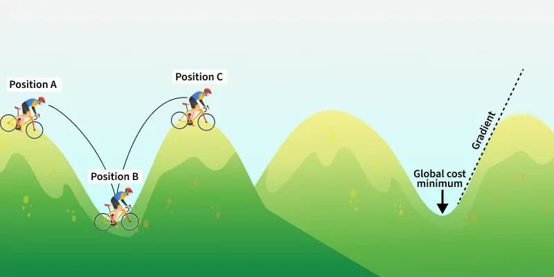
Flat regions and narrow valleys behave very differently. In flat regions, gradients are small, leading to slow progress. In narrow valleys, gradients may be steep in one direction and shallow in another, causing oscillations. Convergence theory explains why momentum-based variants and adaptive methods can stabilise updates by smoothing the optimisation trajectory.
Understanding stability is especially important in high-dimensional spaces, where intuition based on two-dimensional examples breaks down. Theoretical analysis provides a framework for predicting behaviour in these complex settings, reinforcing why mathematical foundations remain relevant even in applied AI workflows.
Convergence Rates in Practical Optimisation
Beyond basic gradient descent, convergence theory extends to many popular variants. Batch gradient descent, stochastic gradient descent, and mini-batch methods each have distinct convergence properties. While batch methods offer cleaner theoretical guarantees, stochastic methods trade some stability for efficiency.
Proofs often show that stochastic gradient descent converges in expectation rather than deterministically. The convergence rate is typically sublinear, meaning improvements slow over time. However, these methods scale well to large datasets and remain dominant in practice.
Adaptive optimisers further complicate analysis by adjusting learning rates dynamically. While empirical performance is strong, theoretical guarantees are still an active research area. For practitioners, exposure to these nuances through an ai course in mumbai can bridge the gap between formal theory and real-world model training.
Why Convergence Theory Matters in Real Applications
It is tempting to treat optimisation algorithms as black boxes that simply work when given enough data and compute. However, convergence failures can be costly. Models that do not converge waste resources, delay projects, and produce unreliable results.
Convergence theory equips practitioners with diagnostic tools. It helps explain why training stalls, why loss values fluctuate, or why different initialisations lead to different outcomes. This understanding enables informed adjustments to learning rates, model architecture, and optimisation strategies.
Conclusion
Gradient descent convergence theory provides the mathematical backbone for one of the most widely used optimisation methods in machine learning. By analysing the relationship between objective function properties, step size selection, and stability, this theory explains both the strengths and limitations of iterative optimisation. While modern tools automate much of the process, a solid grasp of convergence principles remains invaluable. It empowers practitioners to design, tune, and troubleshoot models with confidence, ensuring that optimisation is not just effective, but also reliable and predictable.

